Using metpy for WRF analysis
In this tutorial, we will show you how xWRF enables a seamless integration of WRF data with metpy. In the end, we will have a Skew-T plot at a lat-lon location in the simulation domain. Much of this tutorial was adapted from metpy.
Loading the data
First of all, we load the data and use a simple .xwrf.postprocess() call.
import xwrf

ds = xwrf.tutorial.open_dataset("wrfout").xwrf.postprocess()
ds
<xarray.Dataset> Size: 104MB
Dimensions:                    (y: 340, x: 270, Time: 1, z: 39, x_stag: 271,
                                y_stag: 341)
Coordinates: (12/13)
    XLAT                       (y, x) float32 367kB 22.27 22.31 ... 57.54 57.58
    XLONG                      (y, x) float32 367kB -116.7 -116.6 ... -110.9
    XTIME                      (Time) datetime64[ns] 8B ...
    XLAT_U                     (y, x_stag) float32 369kB 22.25 22.29 ... 57.6
    XLONG_U                    (y, x_stag) float32 369kB -116.7 ... -110.8
    XLAT_V                     (y_stag, x) float32 368kB 22.23 22.28 ... 57.62
    ...                         ...
  * z                          (z) float32 156B 0.9969 0.9899 ... 0.002948
  * Time                       (Time) datetime64[ns] 8B 2099-10-01
  * x                          (x) float64 2kB -4.728e+06 ... -2.307e+06
  * y                          (y) float64 3kB -3.341e+05 ... 2.717e+06
  * x_stag                     (x_stag) float64 2kB -4.733e+06 ... -2.303e+06
  * y_stag                     (y_stag) float64 3kB -3.386e+05 ... 2.721e+06
Data variables:
    Times                      (Time) |S19 19B b'2099-10-01_00:00:00'
    U                          (Time, z, y, x_stag) float32 14MB ...
    V                          (Time, z, y_stag, x) float32 14MB ...
    SINALPHA                   (Time, y, x) float32 367kB 0.5507 ... 0.489
    COSALPHA                   (Time, y, x) float32 367kB 0.8347 ... 0.8723
    QVAPOR                     (Time, z, y, x) float32 14MB ...
    PSN                        (Time, y, x) float32 367kB ...
    air_potential_temperature  (Time, z, y, x) float32 14MB 302.2 ... 501.3
    air_pressure               (Time, z, y, x) float32 14MB 1.009e+05 ... 5.2...
    wind_east                  (Time, z, y, x) float32 14MB -0.8541 ... 12.5
    wind_north                 (Time, z, y, x) float32 14MB -4.625 ... -0.8308
    wrf_projection             object 8B +proj=lcc +x_0=0 +y_0=0 +a=6370000 +...
Attributes: (12/149)
    TITLE:                            OUTPUT FROM WRF V4.1.3 MODEL
    START_DATE:                      2099-08-01_00:00:00
    SIMULATION_START_DATE:           2099-08-01_00:00:00
    WEST-EAST_GRID_DIMENSION:        271
    SOUTH-NORTH_GRID_DIMENSION:      341
    BOTTOM-TOP_GRID_DIMENSION:       40
    ...                              ...
    ISLAKE:                          21
    ISICE:                           15
    ISURBAN:                         13
    ISOILWATER:                      14
    HYBRID_OPT:                      0
ETAC: 0.0Sampling
Then, we sample the dataset at the desired location using pyproj. Let’s use San Francisco for now.
import numpy as np
from pyproj import Transformer, CRS


def sample_wrf_ds_at_latlon(ds, lat, long):
    trf = Transformer.from_crs(CRS.from_epsg(4326), ds.wrf_projection.item(), always_xy=True)
    x, y = trf.transform(long, lat)
    return ds.interp(x=x, y=y, x_stag=x, y_stag=y)
ds_sampled = sample_wrf_ds_at_latlon(ds, 37.773972, -122.431297)
ds_sampled
<xarray.Dataset> Size: 2kB
Dimensions:                    (Time: 1, z: 39)
Coordinates: (12/13)
    XLAT                       float64 8B 37.77
    XLONG                      float64 8B -122.4
    XTIME                      (Time) datetime64[ns] 8B ...
    XLAT_U                     float64 8B 37.77
    XLONG_U                    float64 8B -122.4
    XLAT_V                     float64 8B 37.77
    ...                         ...
  * z                          (z) float32 156B 0.9969 0.9899 ... 0.002948
  * Time                       (Time) datetime64[ns] 8B 2099-10-01
    x                          float64 8B -4.176e+06
    y                          float64 8B 1.394e+06
    x_stag                     float64 8B -4.176e+06
    y_stag                     float64 8B 1.394e+06
Data variables:
    Times                      (Time) |S19 19B b'2099-10-01_00:00:00'
    U                          (Time, z) float64 312B 5.312 6.197 ... 0.7563
    V                          (Time, z) float64 312B -3.233 -3.76 ... -3.614
    SINALPHA                   (Time) float64 8B 0.609
    COSALPHA                   (Time) float64 8B 0.7931
    QVAPOR                     (Time, z) float64 312B 0.01309 ... 3.416e-06
    PSN                        (Time) float64 8B 0.0
    air_potential_temperature  (Time, z) float64 312B 295.8 295.8 ... 497.2
    air_pressure               (Time, z) float64 312B 1.007e+05 ... 5.282e+03
    wind_east                  (Time, z) float64 312B 6.149 7.021 ... 2.802
    wind_north                 (Time, z) float64 312B 0.6446 0.6486 ... -2.406
    wrf_projection             object 8B +proj=lcc +x_0=0 +y_0=0 +a=6370000 +...
Attributes: (12/149)
    TITLE:                            OUTPUT FROM WRF V4.1.3 MODEL
    START_DATE:                      2099-08-01_00:00:00
    SIMULATION_START_DATE:           2099-08-01_00:00:00
    WEST-EAST_GRID_DIMENSION:        271
    SOUTH-NORTH_GRID_DIMENSION:      341
    BOTTOM-TOP_GRID_DIMENSION:       40
    ...                              ...
    ISLAKE:                          21
    ISICE:                           15
    ISURBAN:                         13
    ISOILWATER:                      14
    HYBRID_OPT:                      0
ETAC: 0.0Computation of desired quantities
Now we have to compute the quantities metpy uses for the skewT. For that we have to first quantify the WRF data and then convert the data to the desired units.
import metpy
import metpy.calc as mpcalc
import pint_xarray


ds_sampled = ds_sampled.metpy.quantify()
ds_sampled['dew_point_temperature'] = mpcalc.dewpoint(
    mpcalc.vapor_pressure(ds_sampled.air_pressure, ds_sampled.QVAPOR)
).pint.to("degC")
ds_sampled['air_temperature'] = mpcalc.temperature_from_potential_temperature(
    ds_sampled.air_pressure, ds_sampled.air_potential_temperature
).pint.to("degC")
ds_sampled['air_pressure'] = ds_sampled.air_pressure.pint.to("hPa")
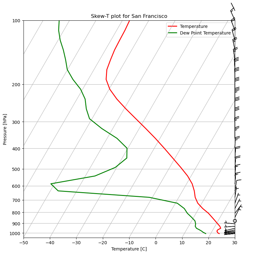
Plotting
Finally, we can create the skew-T plot using the computed quantities.
import matplotlib.pyplot as plt
from metpy.plots import SkewT

# Create a new figure. The dimensions here give a good aspect ratio
fig = plt.figure(figsize=(9, 9))
skew = SkewT(fig)

# Make the dimensions of the data palatable to metpy
ds_sampled = ds_sampled.squeeze()

# Plot the data using normal plotting functions, in this case using
# log scaling in Y, as dictated by the typical meteorological plot
skew.plot(ds_sampled.air_pressure, ds_sampled.air_temperature, 'r', linewidth=2, label='Temperature')
skew.plot(
    ds_sampled.air_pressure, ds_sampled.dew_point_temperature, 'g', linewidth=2, label='Dew Point Temperature'
)
skew.plot_barbs(ds_sampled.air_pressure, ds_sampled.wind_east, ds_sampled.wind_north)

# Make the plot a bit prettier
plt.xlim([-50, 30])
plt.xlabel('Temperature [C]')
plt.ylabel('Pressure [hPa]')
plt.legend().set_zorder(1)
plt.title("Skew-T plot for San Francisco")

# Show the plot
plt.show()